\(\newcommand{\abs}[1]{\left\lvert#1\right\rvert}\) \(\newcommand{\norm}[1]{\left\lVert#1\right\rVert}\) \(\newcommand{\inner}[1]{\left\langle#1\right\rangle}\) \(\DeclareMathOperator*{\argmin}{arg\,min}\) \(\DeclareMathOperator*{\argmax}{arg\,max}\) \(\DeclareMathOperator*{\E}{\mathbb{E}}\) \(\DeclareMathOperator*{\V}{\mathbb{V}}\) \(\DeclareMathOperator*{\x}{\mathbf{x}}\)
G
oogle released Gemma 4 E2B earlier this month (April 2026) as the lightest entry in the family – 2.3B “effective” parameters, 5.1B if you count the per-layer embedding table. It is a sensible candidate for compression research: small enough to instrument on a single CPU, but architecturally rich enough that the usual sins of low-rank approximation and quantization tell different stories on different parts of the model.
This post is a survey of the weight matrices and KV cache, viewed through three lenses – distributional, spectral, and random-matrix-theoretic. The findings change which parts of the model are good targets for which kind of compression.
Notation: $L = 35$ – number of transformer blocks. $d_{model} = 1536$ – hidden size. $d_k$ – head dimension (256 for sliding, 512 for global layers). $\sigma_i$ – $i$th singular value of a weight matrix; $\lambda_i = \sigma_i^2$ – corresponding eigenvalue of $W^T W$.
Architectural sketch
The text decoder has 35 transformer blocks. Each block has standard ingredients with a few twists worth noting up front:
- Hidden size 1536, vocab 262144, embeddings tied to the LM head (verified by
data_ptrequality betweenembed_tokens.weightandlm_head.weight). - Grouped-query attention with 8 query heads and 1 KV head — already a 8× reduction of the cache vs. multi-head.
- Two head-dim regimes: sliding layers use head_dim=256, global layers use head_dim=512. Globals at indices 4, 9, 14, 19, 24, 29, 34. The pattern is
[sliding ×4, global ×1] × 7. - KV sharing:
num_kv_shared_layers=20— only the first 15 blocks compute K/V; layers 15–34 borrow them. Confirmed at runtime: HuggingFace’sDynamicCachematerialises 15 entries for 35 layers, a 57% memory saving over a naive cache. - Wide MLPs in the second half:
intermediate_sizedoubles from 6144 (layers 0–14) to 12288 (layers 15–34). The widening compensates for the missing K/V projections so per-layer parameter counts stay roughly balanced. - PLE (“E2B”) trick: a single shared table
embed_tokens_per_layer [262144, 8960]where 8960 = 35 × 256. Each token’s slice contributes a 256-dim layer-specific signal, injected into the residual stream via per-layer gate/projection/norm. Accounts for ~46% of checkpoint params. - Two RoPE regimes: standard θ=10K on sliding, proportional RoPE (θ=1M,
partial_rotary_factor=0.25) on global — only 25% of dims rotated.
That is the staging. Now to the statistics.
Weights are very nearly Gaussian
Across all 205 projection matrices in the decoder (Q/K/V/O for the 15 KV-owning layers, plus gate/up/down for all 35), the entry-wise distribution is well-approximated by a zero-mean Gaussian with standard deviation in $[0.009, 0.027]$ and excess kurtosis in $[0.1, 10]$ — most matrices sit comfortably in the middle of these ranges. Near-zero entry fraction $(|w| < 1e-4)$ sits between $0.3%$ and $1.1%$, so element-wise pruning isn’t on the table.
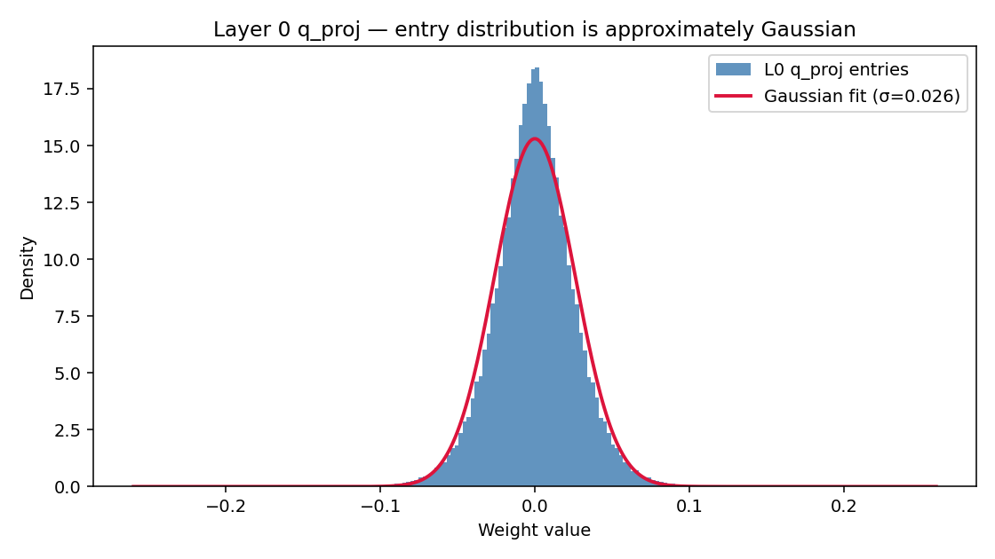
W = get_weight("layers.0.self_attn.q_proj").flatten()
print(W.mean(), W.std())          # ≈ 0, ≈ 0.022 (L0 q_proj specifically;
                                  # project-wide range is [0.009, 0.027])
print(np.abs(W).max())            # ~ 0.25 — tightly clipped during training
The one stark exception is RMSNorm scale. Some norm weights have max-abs values reaching ~900 and excess kurtosis well into the hundreds; others are tame, but the spread is wide. Whatever quantization scheme you apply to projections, keep all norm weights in fp16/bf16 – they are cheap (a few thousand floats per layer) and the outlier-heavy ones would suffer disproportionately under aggressive quantization.
Singular-value decay differs sharply by role
Below is the normalised singular value spectrum for q_proj at seven sample layers:
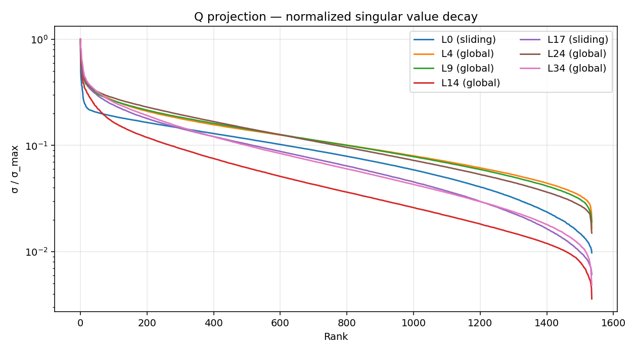
Layer 14 stands out. Its decay is among the steepest in the model — the largest singular value is far larger than the rest of the spectrum — while a layer like 0 or 24 has a much gentler slope.
A summary metric across all 205 weight matrices is stable rank, ||W||_F² / σ_max². It’s robust to noise and gives the effective “rank-1-ness” of a matrix:
![]()
| Role | Stable rank (mean) | Interpretation |
|---|---|---|
| V | ~23 | Top few SVs dominate — looks rank-1-ish |
| Q | ~33 | Top few SVs dominate — looks low-rank |
| K | ~33 | Same range as Q |
| O | ~54 | Energy more spread |
| gate | ~61 | Moderate |
| down | ~137 | Energy widely spread |
| up | ~169 | Most spread of all |
The lowest single stable-rank values sit around 11 (gate at L14) and 14 (Q at L14) – small enough to look like extreme low-rank candidates. Stable rank around 14 sounds like “this matrix is basically rank 14” and tempts you to truncate to the top 14 singular values. That is only correct if the rest of the spectrum is noise – and that is exactly the question random matrix theory can answer cleanly.
Marchenko-Pastur distribution
If you take an $out \times in$ matrix with i.i.d. zero-mean entries of variance $\sigma^2$, and form the sample covariance $(1/N) W^T W$ with $N = max(out, in)$ and $D = min(out, in)$, the Marchenko-Pastur theorem says the eigenvalues of that covariance concentrate on a known interval:
def mp_edges(q, sigma2):
    return sigma2 * (1 - np.sqrt(q)) ** 2, sigma2 * (1 + np.sqrt(q)) ** 2

def mp_density(lam, q, sigma2):
    lo, hi = mp_edges(q, sigma2)
    out = np.zeros_like(lam, dtype=float)
    inside = (lam > lo) & (lam < hi)
    out[inside] = np.sqrt(
        (hi - lam[inside]) * (lam[inside] - lo)
    ) / (2 * np.pi * q * sigma2 * lam[inside])
    return out
The bulk shape depends only on $q = D/N$. Anything above $λ_+ = \sigma^2(1+\sqrt{q})^2$ is structured signal that training carved out beyond what i.i.d. noise would produce. Counting those “signal” eigenvalues gives a cleaner notion of effective rank than energy heuristics.
For Gemma 4’s weights, this is what we see:
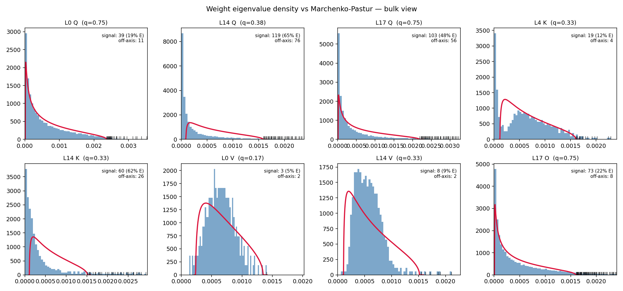
The story splits into three regimes:
Random-like. MLP up and down show a textbook MP bulk. About 5-7% of eigenvalues poke above the upper edge, carrying ~15–20% of energy (up: 15%, down: 20%). The rest of the spectrum is statistically indistinguishable from a trained random matrix.
Bulk-and-spikes. MLP gate, attention K, and O show an MP-shaped bulk plus a moderate signal layer above. K and O carry ~27–29% of their energy in spikes; gate ~23%.
Heavy-tailed. Attention Q and V both sit above the MP edge, but the violation differs in kind. For Q, the bulk itself is deformed: on average 12% of eigenvalues fall below the MP lower edge $λ_-$ (where the law predicts zero), meaning mass has shifted toward zero rather than spreading across $[λ_-, λ_+]$. For V, the bulk respects $λ_-$ – only ~1% of eigenvalues land below it – but V carries a few extremely dominant directions: the top eigenvalue averages 7× the noise floor. So Q’s violation is bulk-deforming; V’s is tail-confined.
A per-layer view of “signal eigenvalues as a fraction of min dim” makes the regime split obvious:
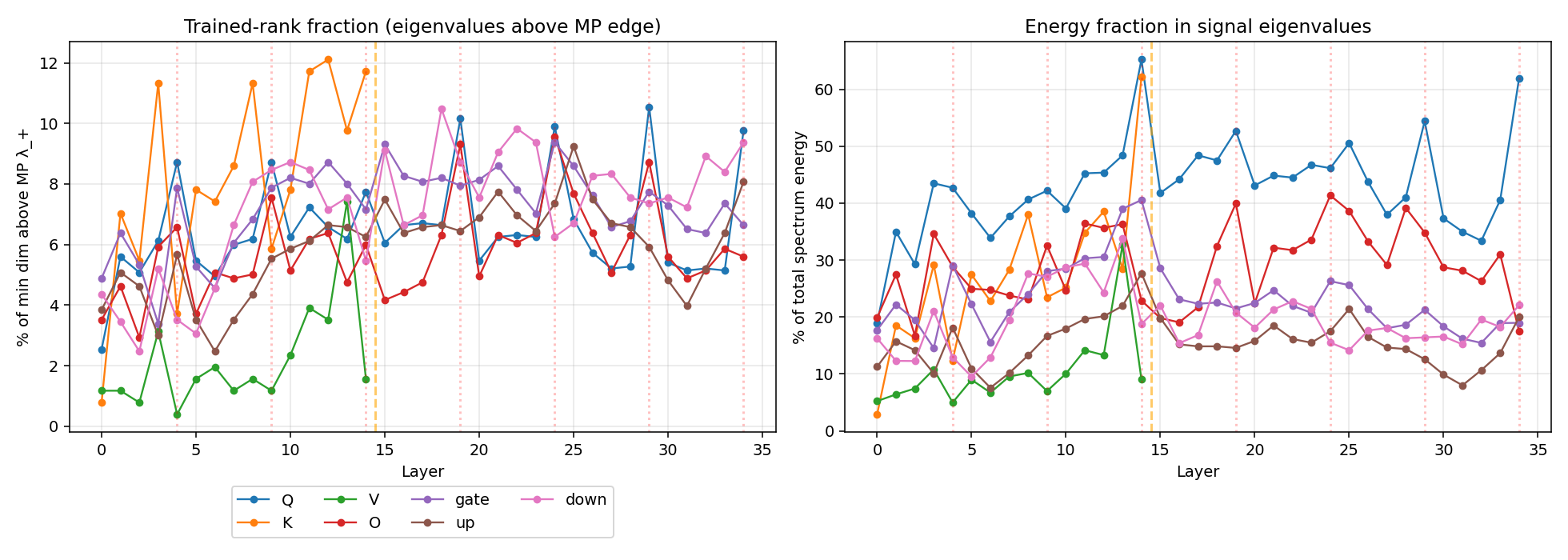
Layer 14 of Q and K both jump up dramatically – at L14, 65% of Q’s spectrum energy is above the MP edge (vs. ~20-40% elsewhere) and 62% of K’s (vs. ~12-30% elsewhere).
The HTSR power-law exponent
Martin & Mahoney’s “Heavy-Tailed Self-Regularization” framework fits a power law to the upper tail of each weight’s eigenvalue spectrum, $p(\lambda) \sim \lambda^{-\alpha}$. Lower $\alpha$ means heavier tail, which in turn means more strongly trained.
Empirical convention: $\alpha \in [2, 4]$ = well-trained, $\alpha > 6$ = under-trained / random-like, with $\alpha \approx 4$-$6$ reading as “approaching random.”
def fit_htsr_alpha(eigvals, top_frac=0.10):
    eigvals = np.sort(eigvals)[::-1]
    n_top = max(int(len(eigvals) * top_frac), 20)
    log_lam = np.log(eigvals[:n_top] + 1e-30)
    log_rank = np.log(np.arange(1, n_top + 1))
    slope, _ = np.polyfit(log_lam, log_rank, 1)
    return 1 - slope
Fitting this to all 205 weight matrices gives:
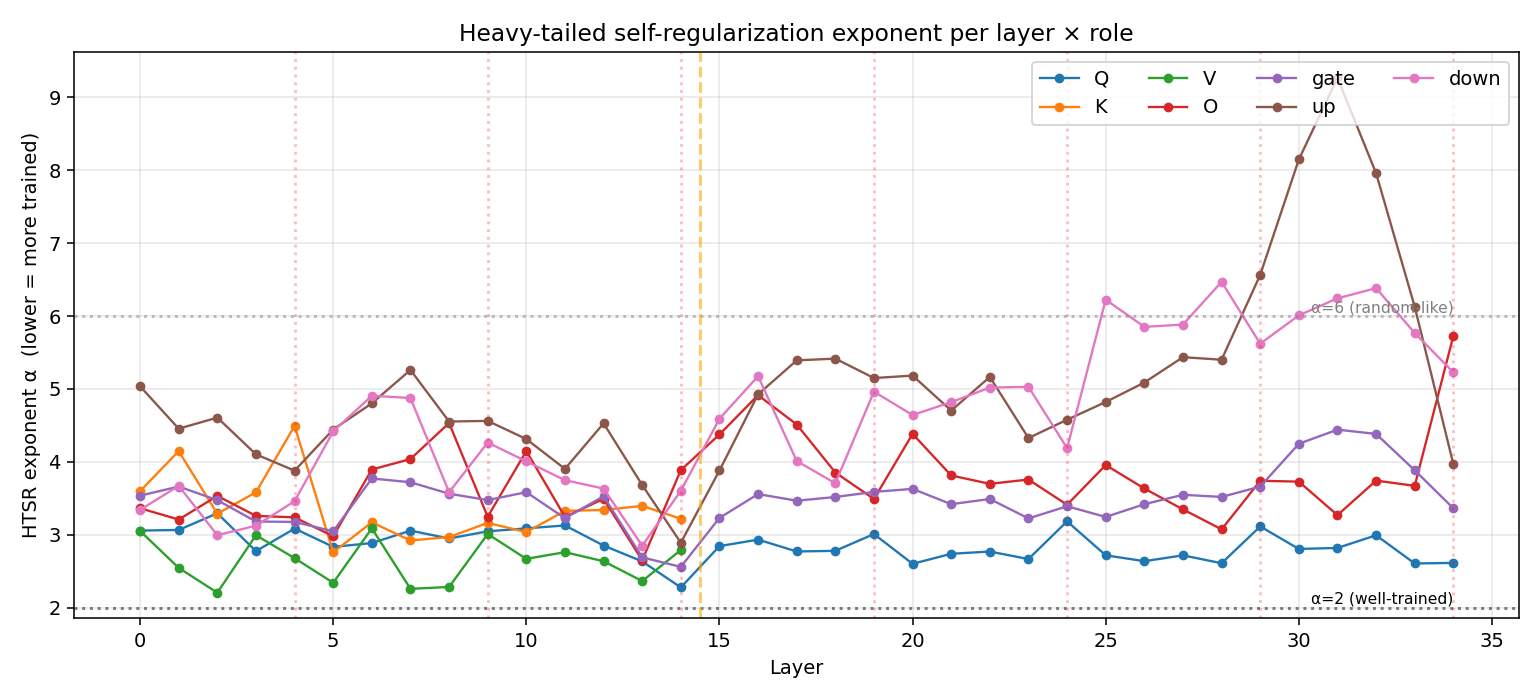
Per-role mean α values:
| Role | α (mean) | Where the minimum sits | Regime |
|---|---|---|---|
| V | 2.65 | layer 2 (α=2.21) | Heavy-tailed |
| Q | 2.86 | layer 14 (α=2.28) | Heavy-tailed |
| gate | 3.50 | layer 14 (α=2.56) | Bulk-and-spikes |
| K | 3.36 | layer 5 (α=2.76) | Bulk-and-spikes |
| O | 3.74 | layer 13 (α=2.65) | Bulk-and-spikes |
| down | 4.64 | layer 13 (α=2.85) | Approaching random |
| up | 5.04 | layer 14 (α=2.89) | Random-like |
So V is the most heavy-tailed role on average, but with the smallest signal count (2.2% of eigenvalues above $λ_+$) and lowest signal energy (10.4%). As established in §3, V’s bulk respects the MP lower boundary; the violation is tail-confined – a handful of extreme outliers reaching 7× the noise floor on average, sitting atop an otherwise passable MP bulk. That makes V a poor fit for hard low-rank truncation: those outliers carry only ~10% of energy, leaving 90% in the bulk with no natural cutoff.
Q on the other hand has both a heavy tail and many spikes — a regime where the model has learned both a few dominant directions and a heavy continuum below them.
Layer 14 in detail:
| Role at L14 | Signal count | Signal energy % | α |
|---|---|---|---|
| Q | 119 (7.7%) | 65.2% | 2.28 (model’s lowest Q) |
| K | 60 (11.7%) | 62.2% | 3.22 (not the lowest K) |
| V | 4 (1.6%) | 9.0% | 2.79 |
| O | 92 (6.0%) | 22.9% | 3.89 |
| gate | 110 (7.2%) | 40.6% | 2.56 (model’s lowest gate) |
| up | 96 (6.3%) | 27.7% | 2.89 (model’s lowest up) |
| down | 84 (5.5%) | 18.8% | 3.60 |
L14 is the most-trained layer for Q, gate, and up simultaneously. K’s most-heavy-tailed point is actually at layer 5, but its L14 spike count (60) and signal energy (62%) are both the highest in the model. So L14 is special, but for the MLP and Q specifically – not for K or V’s heavy-tail signature, both of which peak elsewhere.
Cross-layer subspace structure
Singular value spectra describe one matrix at a time. To see how layers relate to each other, the natural object is the subspace each weight defines in the hidden space $R^{1536}$. For each Q projection, take the top-64 right singular vectors (an orthonormal basis for the dominant input subspace), then compare bases pairwise via mean cos² of principal angles. Both the unweighted version, $mean(cos^2θ_l)$, and a $\sigma^2$-weighted variant (which downweights noise directions by the geometric mean of the corresponding singular values) tell the same story:
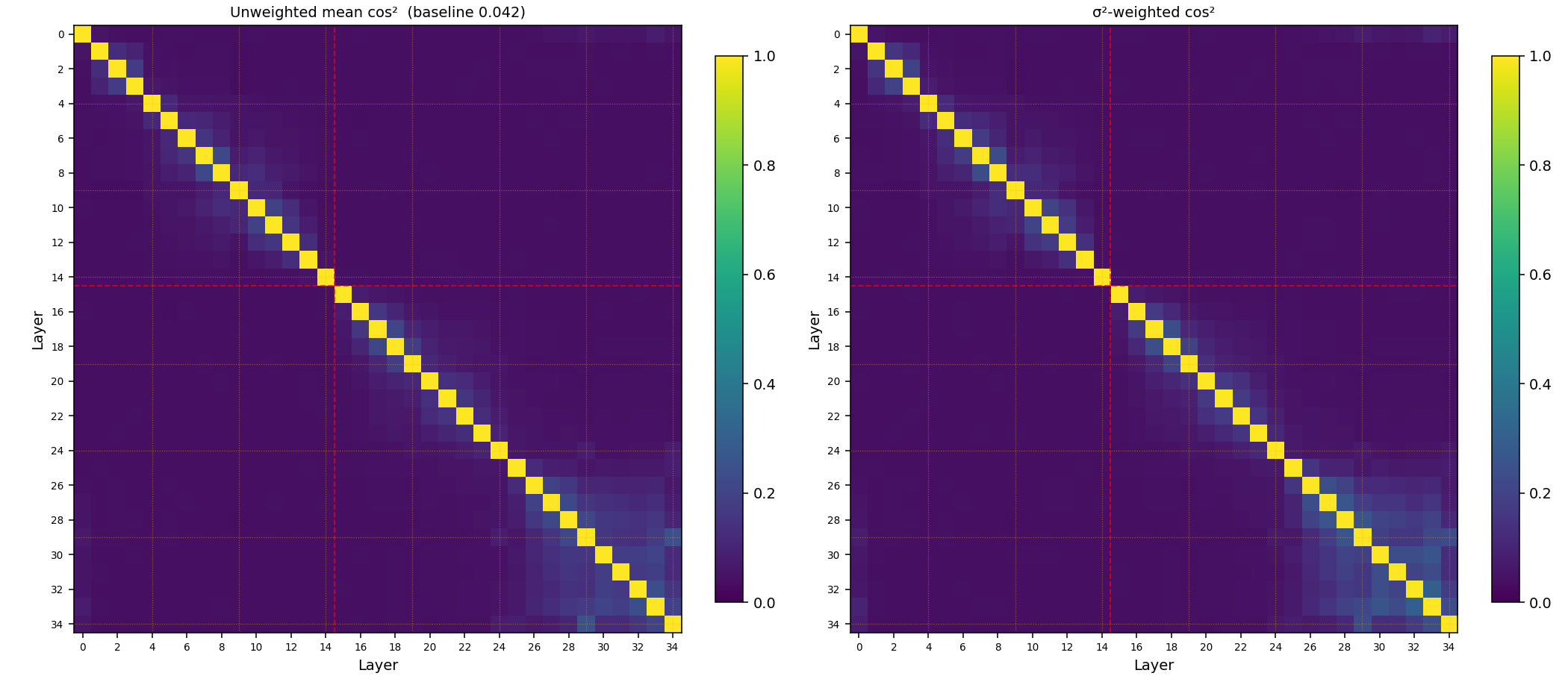
Visually the structure is faint, but it sharpens once you anchor against the random baseline. Two random 64-dim subspaces in $R^{1536}$ have expected mean cos² of $64/1536 \approx 0.042$. So 0.042 is the floor; off-diagonal cells should be read as multiples of it.
| Pair type | Unweighted | $\sigma^2$-weighted | × baseline |
|---|---|---|---|
| sliding ↔ adjacent sliding (|i-j|=1) | 0.157 | 0.182 | 3.8× |
| global ↔ adjacent sliding | 0.118 | 0.133 | 2.8× |
| sliding ↔ far sliding (|i-j|≥5) | 0.045 | 0.046 | 1.1× |
| within first half (0..14, off-diag mean) | 0.063 | 0.066 | 1.5× |
| within second half (15..34, off-diag mean) | 0.076 | 0.083 | 1.8× |
| across halves (first ↔ second) | 0.042 | 0.043 | 1.0× — exactly random |
Three concrete findings, in order of strength:
- The KV-share boundary at layer 15 is a sharp subspace boundary. Cross-half mean overlap sits exactly at the random baseline. The first and second halves of the decoder use Q-subspaces that are essentially uncorrelated — the second half is not a continuation of the first, it’s pulling on genuinely different directions of the hidden space.
- Local sliding alignment is real but short-range. Adjacent slidings share 3.8× more subspace energy than random; five layers away, alignment is back at baseline. The “block” of sliding structure is a 1-2 layer band, not a wide block of similar layers.
- Globals are mildly less aligned with their neighbours than slidings are with each other — 2.8× vs 3.8×. They’re outliers, but only modestly so.
The $\sigma^2$-weighted variant agrees with the unweighted in direction and magnitude (slightly amplified differences), so the structure isn’t an artifact of including noise directions in the basis.
KV cache properties at runtime
Weights tell you what the network can do; activations tell you what it does. A single forward pass over a 1500-token prose prompt, with attn_implementation="eager" to expose attention weights, gives the runtime picture.
Two findings stand out — both with direct compression implications.
KIVI’s hypothesis is inverted for K. KIVI (Liu et al.) observed that K cache outliers are channel-aligned — a few channels carry disproportionate magnitude across all tokens — while V cache outliers are token-aligned. Their recipe: per-channel quantization for K, per-token for V.
For Gemma 4:
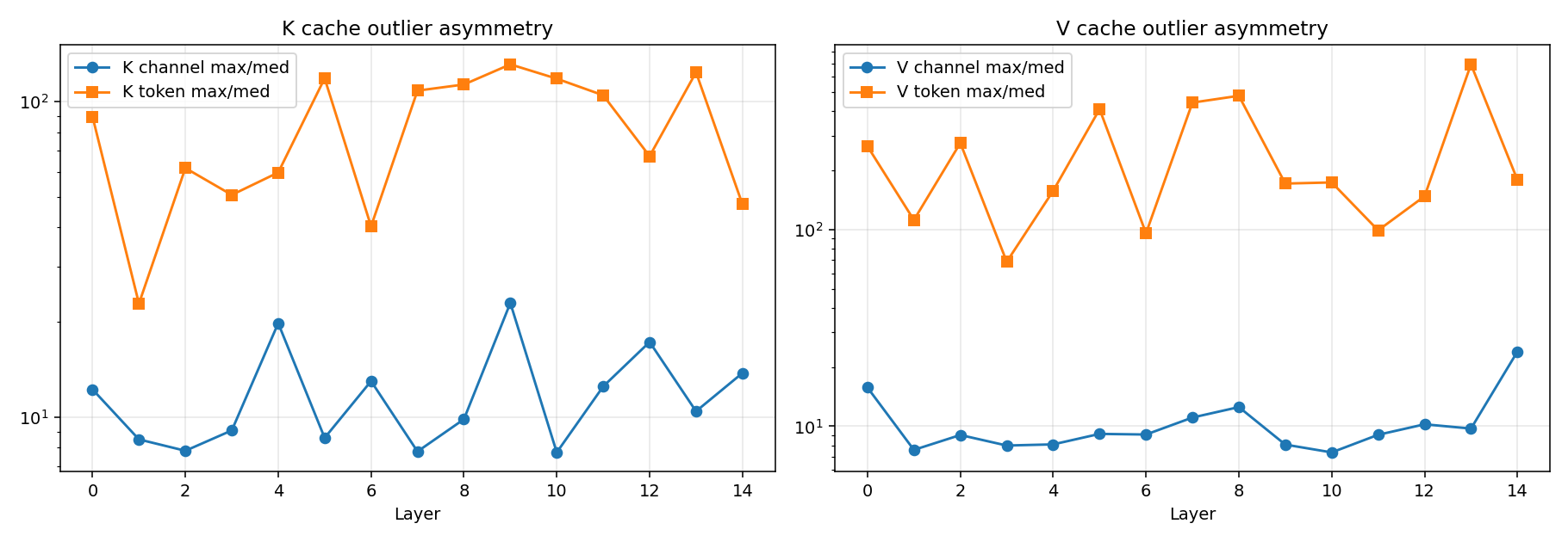
V matches KIVI’s prediction: token outliers dominate channel outliers in 100% of (layer × prompt) combinations across prose, code, and structured prompts. K behaves like V here, not like KIVI’s prediction for K — K’s worst token outlier also exceeds its worst channel outlier in 100% of cases. The KIVI asymmetry is gone; both caches look token-aligned, and the inversion for K is universal rather than a tendency. A plausible mechanism: Gemma 4 applies RMSNorm to K before RoPE, normalising each token’s K vector. This bounds per-channel cross-token spread but leaves room for within-token channel imbalance, which RoPE then amplifies into a few high-magnitude channels per token. For Gemma 4, use per-token K quantization, not the standard per-channel scheme.
The V cache uses more of head_dim than the V weight spectrum suggests. v_proj looks rank-1-friendly on the weight side (top SV is 2–5× the rest, low stable rank), and yet the V cache itself has Shannon-entropy effective rank 140/256 (55%) for sliding layers and 318/512 (62%) for global layers. (Shannon-entropy effective rank, defined as $e^{H(p)}$ over normalised singular values, measures the flatness of the spectrum.) Weight SVD lies as a predictor of cache compressibility. Real V activations span more of head_dim than the weights’ SV decay suggests, because the input distribution exercises directions the weights’ Frobenius geometry de-emphasises.
A complementary view via MP on the cache itself:
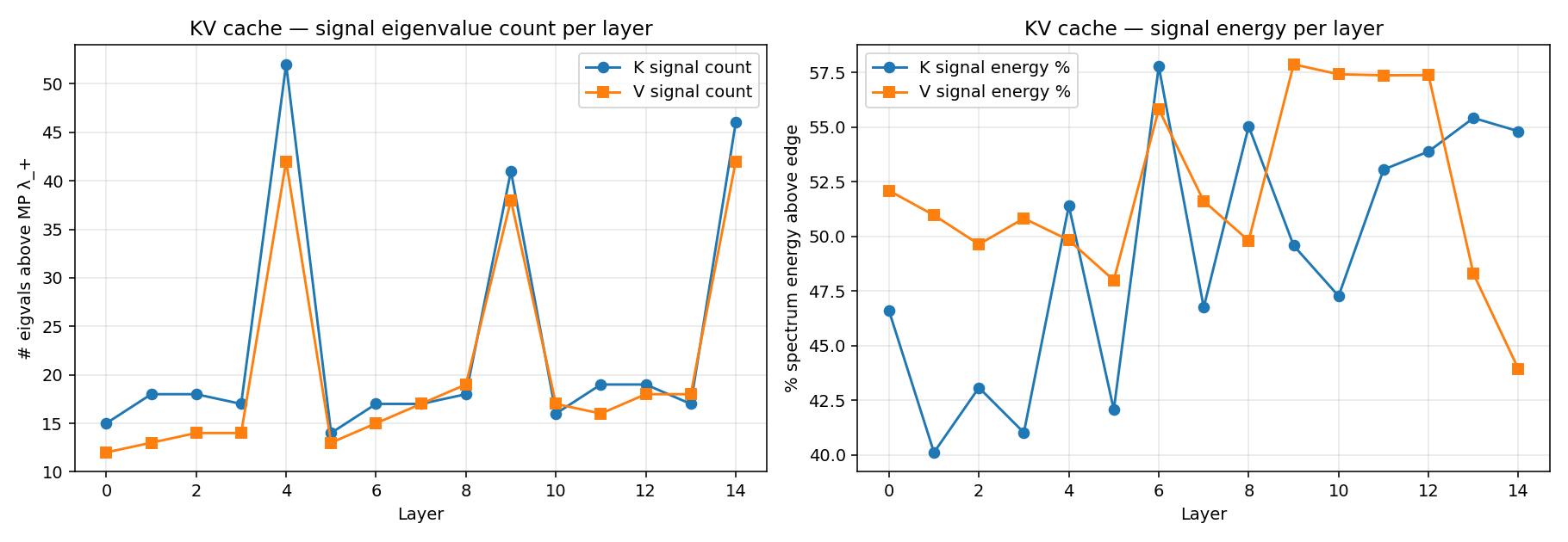
V’s signal eigenvalue count above the MP edge is in the mid-teens for sliding layers and ~40 for globals — meaning the cache’s spectrum is broad (high Shannon eff-rank) but only a fraction of it sits above the i.i.d. noise floor. Both metrics agree on the same qualitative point: low-rank V-cache compression should be calibrated on activations, not weights. The actual achievable rank reduction depends on which loss you’re willing to take, and is best determined by a reconstruction-error sweep rather than read off either rank metric directly.
A note on attention sinks: Gemma 4 puts only 0.4% of attention mass on the first 4 tokens at global layers – confirming the model lacks the strong attention-sink behaviour StreamingLLM relies on. Sliding layers actually carry slightly more sink mass (1.6% on prose, up to 2.5% on structured prompts), and a handful of late-layer heads (notably L27-L33 head 4) reach ~5% sink mass individually. So “keep the first few tokens + recent window” is not a free win for this model – and the heads that do sink-attend are scattered across layers and heads rather than concentrated, so token-eviction schemes need head-level analysis instead of a uniform rule.
Cross-layer KV cache overlap
Earlier we looked at how Q weights relate across layers. The natural compression-side analogue is: do the K and V caches — the actual activation tensors stored at inference time — share subspace structure across layers? If they did, you could store one shared basis per cache type and per-layer coefficients, replacing n × T × head_dim floats with head_dim × k + n × T × k (~88% saving for typical k).
For each pair of computing layers (i, j) with the same head_dim, take the cache tensor [T, head_dim] from a forward pass on the realistic prose, compute the top-k PCA basis of layer i’s cache, then measure what fraction of layer j’s cache variance lives in that basis. This is asymmetric (anchor → query) and directly compression-relevant: if i’s basis explains 90% of j, you can store j in i’s subspace at 10% reconstruction error.
Using $k = 32$ for sliding (head_dim=256, ≈12.5% — close to the average MP signal count of ~16) and $k = 48$ for global (head_dim=512, ≈9.4% — close to the average MP signal count of ~41):
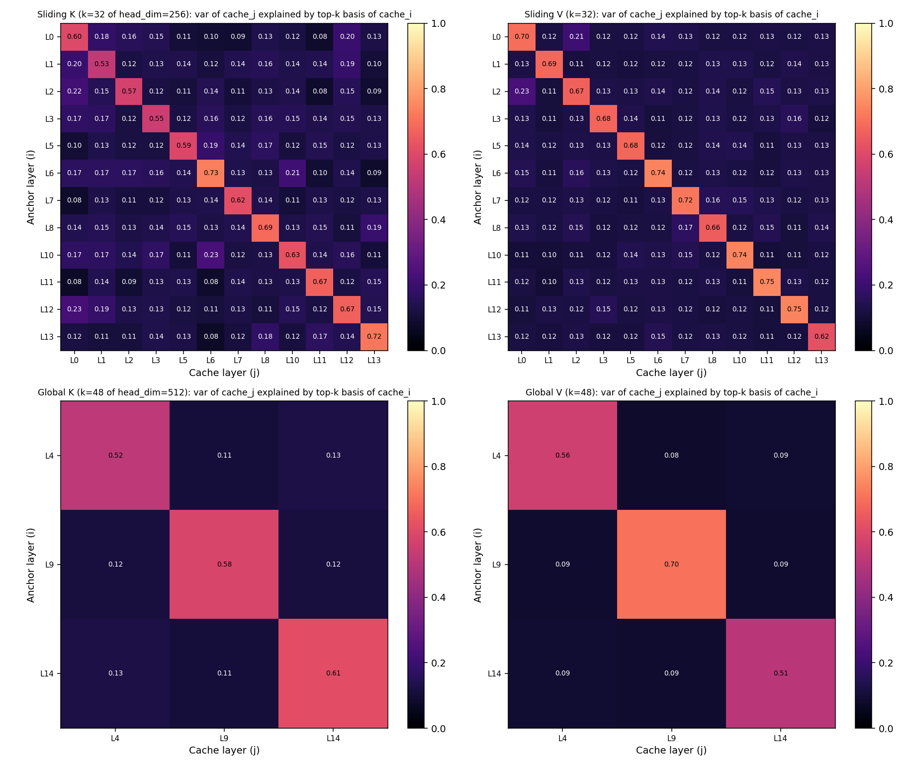
The picture is decisively negative for naive cross-layer factorisation:
- Diagonals (a layer’s own basis explaining its own cache) capture 53–75% of variance — the expected ceiling at this
k. - Off-diagonals (one layer’s basis explaining another’s cache) capture only 8–23%, with most pairs sitting in 0.10–0.15. That’s 1.5–2× the random baseline (random projections from a
k-dim subspace into ahead_dim-dim cache would explaink/head_dim = 12.5%or9.4%of variance for pure-noise data) — meaningfully above noise, but nowhere near “shareable.” - Best anchor’s mean variance explained across the group: 0.18–0.29. Not enough to share without losing most of the cache.
So K and V caches do not live in a shared subspace across layers. Each computing layer has carved out its own ~k-dim slice of head_dim space, and those slices are nearly orthogonal between layers. Cross-layer cache factorisation is ruled out as a compression scheme on Gemma 4 — the only path to additional KV memory savings is per-layer (rank truncation calibrated on activations, or per-token / per-channel quantization as already discussed).
This dovetails with the earlier finding: combined with the sharp Q-subspace discontinuity at the layer-15 KV-share boundary, it means both the weights and the activations of different layers are pulling on genuinely different directions. The model uses depth to access different parts of representation space, not to refine the same directions over and over. That’s bad news for compression schemes that bet on cross-layer redundancy, and good news for understanding what the model is actually doing with its depth.
Opportunities for compression
The RMT lens collapses three observations into a per-role recipe:
| Role | Regime | Recommendation |
|---|---|---|
MLP up, down |
Random-like (α≈5) | Either Gavish-Donoho hard-thresholded SVD, or spike + sketch: keep the ~100 signal eigenvalues exactly, replace the MP bulk with a seeded random matrix of matching $\sigma^2$. The bulk is statistically reproducible noise — doesn’t need to be stored verbatim. |
MLP gate |
Bulk-and-spikes | Standard rank-truncated SVD around the MP threshold (~75 signal directions). Quantize residuals. |
Attention K, O |
Bulk-and-spikes | Same; K is well-suited to per-token quantization (KIVI inverted). |
Attention Q, V |
Heavy-tailed (HTSR) | Avoid pure low-rank truncation. No clean noise floor — every cut loses signal. Use quantization-only or activation-aware decomposition (ASVD/FWSVD). |
| Layer 14 (especially Q, gate, up) | Most-trained | Reserve highest precision; do not aggressively reduce rank. |
| RMSNorm weights | Outlier-heavy | Keep in bf16/fp16. They cost nothing. |
| KV cache (V) | Shannon eff-rank ~55–62% of head_dim; ~15–40 signal eigenvalues above MP edge; no cross-layer overlap | Per-layer rank truncation calibrated on activations; reconstruction-error sweep to pick the cut. Cross-layer factorisation does not work. |
| KV cache (K) | Token-aligned outliers; no cross-layer overlap | Per-token quantization (against KIVI’s published recipe). Cross-layer factorisation does not work. |
Two specific experiments would close the loop:
- Spike + sketch on a representative MLP up/down — pick one layer, factor out the top-100 eigenpairs, replace the bulk with a seeded random matrix of the right scale, measure end-to-end loss change. The MP fit is clean enough that this should almost work without finetuning.
- HTSR quality control — fit α at every layer, refuse low-rank for any matrix with α < 4. This is a 100-line guard rail against destroying training signal in heavy-tailed weights.
TL;DR
Five findings:
-
Weights are near-Gaussian. The exception is RMSNorm scale — outliers reaching ×900 — keep those in full precision regardless of what you do to projections.
-
Three spectral regimes. MLP
up/downare random-like (5–7% of eigenvalues above the noise floor, carrying 15-19% of energy).gate,K,Ohave a clean MP bulk plus moderate signal (23–29% signal energy).QandVare heavy-tailed but differently: Q’s bulk is deformed — 12% of eigenvalues fall below the MP lower edge, where the law predicts zero; V’s bulk respects the MP boundary but carries a handful of extreme outliers (top eigenvalue 7× the noise floor on average). -
Layer 14 is the most-trained layer for Q, gate, and up simultaneously. Reserve highest precision here.
-
KV cache. K outliers are token-aligned, not channel-aligned as KIVI assumes — per-token K quantization is correct for this model. V’s weight spectrum is a misleading proxy for cache compressibility: V activations span 55–62% of head_dim at runtime despite the weight’s low stable rank (~23). Calibrate on activations, not weights.
-
No cross-layer sharing. Q subspaces are orthogonal across the layer-15 KV-share boundary (mean cos² at the random baseline 0.042). K and V caches are similarly orthogonal across layers — cross-layer factorisation is ruled out.