Import MNIST
Let’s get $7000$ examples of length $784 = 28\times 28$ of flattened grayscale square images of handwritten digits, stacked as a tuple of $(X,Y)$ with Python shapes $(70000, 784)$ and $(70000,).$
mnist = fetch_openml("mnist_784", return_X_y=True)
Convert them to allowed formats and do the train-test $(5:2)$ split.
X = np.float32(mnist[0] / 256)  # (70000, 784)
Y = np.int64(mnist[1])  # (70000,)
x_train, y_train, x_valid, y_valid = X[:50000, :], Y[:50000], X[50000:, :], Y[50000:]
Take a look at the first training example!
plt.imshow(x_train[0].reshape((28, 28)), cmap="gray")

DataLoader
Some technical steps
- Convert the data to “torch tensors”
- Form a DataLoader (to simplify the iteration process over batches)
Notice that no shuffling is required for the validation data
x_train, y_train, x_valid, y_valid = map(
    torch.tensor, (x_train, y_train, x_valid, y_valid)
)
train_ds = TensorDataset(x_train, y_train)
valid_ds = TensorDataset(x_valid, y_valid)
train_dl = DataLoader(train_ds, batch_size=64, shuffle=True)
valid_dl = DataLoader(valid_ds, batch_size=128)
Model, Optimizer & Loss
Lets design the NN architecture by subclassing nn.Module , which manages the network parameters/weights, their gradients, etc. Create a simple linear layer self.lin = nn.Linear(784, 10) which implicitly is equivalent to creating a $784\times 10$ matrix of weights and a $10$-dim bias vector
self.weights = nn.Parameter(torch.randn(784, 10) / math.sqrt(784))
self.bias = nn.Parameter(torch.zeros(10))
Both parameters are initially random, Xavier initialized, but need to be determined eventually. For now, let’s not add any nonlinearities. Also incorporate the forward step, which will multiply the input by the matrix and add the bias, xb @ self.weights + self.bias . Hence we have
class FeedForward(nn.Module):
  def __init__(self):
    super().__init__()
    self.lin = nn.Linear(784, 10)

  def forward(self, xb):
    return self.lin(xb)

model = FeedForward()
Pick the optimizer and the learning rate.
opt = optim.Adam(model.parameters(), lr=.001)
Specify the loss. F.cross_entropy combines negative log likelihood loss and log softmax activation and works well for classification purposes.
loss_func = F.cross_entropy
Training
Iterate over all training images $15$ times, each time sampling batches from DataLoader.
For each batch,
- Make a prediction
model(xb), which propagatesxbforward. - Compute the loss
loss_func(pred, yb) - Propagate backwards:
- Update the gradients
- Optimize the weights, i.e. for each parameter
pdop -= p.grad * lr - Reset the gradient back to $0$ so it is ready for the next batch
for epoch in range(15):
  for xb, yb in train_dl:
    pred = model(xb)
    loss = loss_func(pred, yb)

    loss.backward()
    opt.step()
    opt.zero_grad()
  print(loss_func(model(xb), yb))
Validation
Easy to check the validation loss too (the lines model.train() and model.eval() ensure appropriate behavior in more complex cases)
for epoch in range(15):
    model.train()
    for xb, yb in train_dl:
        pred = model(xb)
        loss = loss_func(pred, yb)

        loss.backward()
        opt.step()
        opt.zero_grad()

    # Validation
    model.eval()
    with torch.no_grad():
        valid_loss = sum(
            loss_func(model(xb), yb).tolist() for xb, yb in valid_dl
        ) / len(valid_dl)
Can also plot both losses over epochs

Make a prediction
Plot a few validation images
fig = plt.figure(figsize=(3, 3))
rows, cols = 3, 3
for i in range(0, cols * rows):
    fig.add_subplot(rows, cols, i + 1)
    plt.imshow(x_valid[i].reshape((28, 28)), cmap="gray")
plt.show()
print(torch.argmax(model(x_valid[0:9]), axis=1).reshape(3, 3))
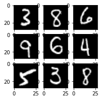 vs $\begin{matrix} [3, 8, 6]\\ [9, 6, 4]\\ [5, 3, 8] \end{matrix}$
CNN
Can use a Convolutional NN instead. Our inputs are $28\times 28\times 1$, where $1$ is the # of channels (only gray).
The first two arguments of Conv2d are in_channels=1 and out_channels=16.
A useful formula for keeping track of dimensions is
\[n_{out} = \frac{n_{in} - k + 2p}{s} + 1\]where $n$ is image’s spatial dimension (height or weight).
Conv2d(1,16,3,2,1): 28x28x1 (28-3+2)/2+1 = 14.5 14x14x16Conv2d(16,16,3,2,1): 14x14x16 (14-3+2)/2+1 = 7.5 7x7x16Conv2d(16,10,3,2,1): 7x7x16 (7-3+2)/2+1 = 4 4x4x10avg_pool2d(xb,4): 4x4x10 1x10
class CNN(nn.Module):
    def __init__(self):
        super().__init__()
        self.conv1 = nn.Conv2d(1, 16, kernel_size=3, stride=2, padding=1)
        self.conv2 = nn.Conv2d(16, 16, kernel_size=3, stride=2, padding=1)
        self.conv3 = nn.Conv2d(16, 10, kernel_size=3, stride=2, padding=1)

    def forward(self, xb):
        xb = xb.view(-1, 1, 28, 28)
        xb = F.relu(self.conv1(xb))
        xb = F.relu(self.conv2(xb))
        xb = F.relu(self.conv3(xb))
        xb = F.avg_pool2d(xb, 4)
        return xb.view(-1, xb.size(1))

model = CNN()
Full Code for CNN
from sklearn.datasets import fetch_openml
import numpy as np
import matplotlib.pyplot as plt
import torch
from torch.utils.data import TensorDataset
from torch.utils.data import DataLoader
from torch import nn
from torch import optim
import torch.nn.functional as F

mnist = fetch_openml("mnist_784", return_X_y=True)
X = np.float32(mnist[0] / 256)  # (70000, 784)
Y = np.int64(mnist[1])  # (70000,)
x_train, y_train, x_valid, y_valid = X[:50000, :], Y[:50000], X[50000:, :], Y[50000:]
plt.imshow(x_train[0].reshape((28, 28)), cmap="gray")

x_train, y_train, x_valid, y_valid = map(
    torch.tensor, (x_train, y_train, x_valid, y_valid)
)
train_ds = TensorDataset(x_train, y_train)
valid_ds = TensorDataset(x_valid, y_valid)
train_dl = DataLoader(train_ds, batch_size=64, shuffle=True)
valid_dl = DataLoader(valid_ds, batch_size=128)


class CNN(nn.Module):
    def __init__(self):
        super().__init__()
        self.conv1 = nn.Conv2d(1, 16, kernel_size=3, stride=2, padding=1)
        self.conv2 = nn.Conv2d(16, 16, kernel_size=3, stride=2, padding=1)
        self.conv3 = nn.Conv2d(16, 10, kernel_size=3, stride=2, padding=1)

    def forward(self, xb):
        xb = xb.view(-1, 1, 28, 28)
        xb = F.relu(self.conv1(xb))
        xb = F.relu(self.conv2(xb))
        xb = F.relu(self.conv3(xb))
        xb = F.avg_pool2d(xb, 4)
        return xb.view(-1, xb.size(1))


model = CNN()
opt = optim.Adam(model.parameters(), lr=0.001)
loss_func = F.cross_entropy

# Training
for epoch in range(15):
    model.train()
    for xb, yb in train_dl:
        pred = model(xb)
        loss = loss_func(pred, yb)

        loss.backward()
        opt.step()
        opt.zero_grad()

    # Validation
    model.eval()
    with torch.no_grad():
        valid_loss = sum(
            loss_func(model(xb), yb).tolist() for xb, yb in valid_dl
        ) / len(valid_dl)
    print(epoch, valid_loss)

# True vs Pred
fig = plt.figure(figsize=(3, 3))
rows, cols = 3, 3
for i in range(0, cols * rows):
    fig.add_subplot(rows, cols, i + 1)
    plt.imshow(x_valid[i].reshape((28, 28)), cmap="gray")  # True
plt.show()
print(torch.argmax(model(x_valid[0:9]), axis=1).reshape(3, 3))  # Pred