Logistic Regression vs AutoML

Let’s compare logistic regression vs AutoGluon, an easy-to-implement AutoML library!

Profile pic

We’ll use spambase data from UCI ML Repository which has $4601$ examples, $57$ features and $0/1$ (no-spam/spam) labels to find out which algorithm is better at detecting spam.

Snapshot of data

#	$X_1$	$X_2$	$X_2$	$\cdots$	$X_{56}$	$X_{57}$	$Y$
0	$.00$	$.64$	$.64$	$\cdots$	$61$	$278$	$1$
1	$.21$	$.28$	$.50$	$\cdots$	$101$	$1028$	$1$
$\vdots$	$\vdots$	$\vdots$	$\vdots$	$\ddots$	$\vdots$	$\vdots$	$\vdots$
4600	$.00$	$.00$	$.65$	$\cdots$	$5$	$40$	$0$

To keep it simple, let’s ignore the data aspects (class imbalance, normalization, etc).

Logistic Regression

We’ll implement a logistic regression with regularization from scratch (using numpy only).

Import Spambase Data

First import the data, change encoding $0/1$ to $-1/1$ for convenience and do train-test split.

import numpy as np
np.random.seed(1)
data = np.loadtxt("https://archive.ics.uci.edu/ml/machine-learning-databases/"
                  + "spambase/spambase.data", delimiter=',')
data = np.random.permutation(data)
data[:, -1] = (lambda x: x*2 - 1)(data[:, -1])  # switch to -1/1

train_y, test_y = data[: 3000, -1:], data[3000:, -1:]  # (3000, 1), (1601, 1)
train_x, test_x = data[: 3000, :-1], data[3000:, :-1]  # (3000, 57), (1601, 57)

Before we proceed, let’s do a very basic feature engineering step: add a column of $1$’s (intercept term) and an extra “indicator” feature that is $1$ if the corresponding $x$ is positive and $0$ otherwise, so that $[3,0,1]$ will turn to $[1, 3, 0, 1, 1, 0, 1]$.

def phi(x):
    ''' adds a column of ones
        and all second-order combinations of features
    '''
    m = x.shape[0]
    x1 = np.hstack((np.ones((m, 1)), x))
    x1 = np.hstack((x1, (x > 0).astype(float)))
    return x1

Loss & Optimizer

It helps to write down the loss, the gradient of the loss, and the Hessian of the loss for logistic regression. The $\ell_2$-penalized loss is ($m$ is sample size, $n$ is dimensionality)

\[\begin{align*} L &= \left[\sum_{i=1}^m \ln(1+e^{-y_i\mathrm{x_i}' \mathrm{w}})\right] + \frac{\lambda}{2}\sum_{j=2}^n w_j^2 \end{align*}.\]

Note that the first weight is not penalized since it corresponds to the intercept. The gradient and Hessian are

\[\begin{align*} \nabla_\mathrm{w} L &= - \left[\sum_{i=1}^m (1-s_i)y_i \mathrm{x}_i'\right] + \lambda\mathrm{w}^* \\ \nabla_\mathrm{w}^2 L &= \left[\sum_{i=1}^m s_i(1-s_i)\mathrm{x}_i\mathrm{x}_i'\right] + \lambda I^*_n \end{align*}\]

where

$s_i = (1+e^{-y_i\mathrm{x}'_i \mathrm{w}})^{-1},\qquad \mathrm{w}^* = \begin{bmatrix} 0 & w_2 & \cdots & w_n \end{bmatrix}', \qquad I^*_n = \begin{bmatrix} 0 & 0 & \cdots & 0 \\ 0 & 1 & \cdots & 0 \\ \vdots & \vdots & \ddots & \vdots \\ 0 & 0 & \cdots & 1 \end{bmatrix}$.

def lrloss(w, x, y, lmbda):
    ''' logistic loss '''
    wstar = w.copy()
    wstar[0] = 0
    return (np.sum(np.log(1+np.exp(-y*(x@w))), 0).T
            + .5*lmbda*np.sum(wstar*wstar))[0]

def lrgrad(w, x, y, lmbda):
    ''' logistic gradient '''
    s = 1/(1+np.exp(-y*(x@w)))
    wstar = w.copy()
    wstar[0] = 0
    return -np.sum((1-s)*x*y, 0)[:, np.newaxis] + lmbda*wstar

def lrhess(w, x, y, lmbda):
    ''' logistic hessian '''
    s = 1/(1+np.exp(-y*(x@w)))
    istar = np.eye(w.shape[0])
    istar[0, 0] = 0
    return x.T@np.diag((s*(1-s))[:, 0])@x + lmbda*istar

Optimization

To estimate the weights, let’s implement a Newton-Raphson optimizer,

\[\begin{align*} \mathrm{w}_{t+1} = \mathrm{w}_t - H^{-1}_{\mathrm{w}_t} g_{\mathrm{w}_t} \end{align*},\]

where $H$ is the Hessian matrix and $g$ is the gradient vector.

This method is relatively straightforward, except when it doesn’t work.

We’ll check if the loss decreased after each iteration to alternate b/w gradient and Newton steps. Each time a second-order step does not decrease the loss, double the step size and try taking a gradient step. If it also fails, keep halving the step size until gradient descent succeeds (leads to smaller loss). As soon as it succeeds, return to second-order steps. Once the step sizes become too small, we are done.

(not a great implementation but demonstrates the idea)

def newton(w, fn, gradfn, hessfn):
    ''' newton-raphson optimizer'''
    oldf = fn(w)
    eta = 1
    while True:
        g = gradfn(w)
        h = hessfn(w)
        neww = w - np.linalg.solve(h, g)  # newton's step
        newf = fn(neww)
        if newf >= oldf:                  # failed to decrease the loss :(
            eta *= 2                      # double the step size
            while eta > 1e-10:
                neww = w - eta*g          # gradient step
                newf = fn(neww)
                if newf < oldf:           # exit if loss decreased!
                    break
                eta *= .5                 # o/w keep halving
            if eta < 1e-10:               # finish if step size too small
                return w
        oldf = newf
        w = neww

Train time!

We should be able to train the model now!

def trainlr(x, y, lmbda):
    ''' training to produce w estimate '''
    w0 = np.zeros((x.shape[1], 1))  # initiating at zero works well for LR
    return newton(w0, lambda w: lrloss(w, x, y, lmbda),
                  lambda w: lrgrad(w, x, y, lmbda),
                  lambda w: lrhess(w, x, y, lmbda))

def lrerrorrate(x, y, w):
    ''' share of incorrectly classified '''
    return np.sum(y*x@w < 0)/y.shape[0]

lmb = .1
mytrain_x, mytest_x = phi(train_x), phi(test_x)
myw = trainlr(mytrain_x, train_y, lmb)
print(lrerrorrate(mytest_x, test_y, myw))

Which gives a training accuracy of about $5.2\%$ !

Profile pic

Cross-Validation

Let’s implement 3-fold cross-validation and plot the cv error as a function of lambda.

def xvalideval(x, y, lmbda):
    ''' validation error '''
    nfold = 3
    px = phi(x)
    m = x.shape[0]
    splits = np.linspace(0, m, nfold+1).astype(int)
    v = 0
    for low, high in zip(splits[0:-1], splits[1:]):
        # validation bucket, from low to high
        validx = px[low:high, :]
        validy = y[low:high, :]
        # training bucket, everything else
        trainx = np.vstack((px[:low, :], px[high:, :]))
        trainy = np.vstack((y[:low, :], y[high:, :]))

        v += lrerrorrate(validx, validy, trainlr(trainx, trainy, lmbda))
    return v

ls = np.logspace(-4, 2, 10)
xverr = ls.copy()
bestv, bestl = None, None
for i, l in enumerate(ls):
    xverr[i] = xvalideval(train_x, train_y, l)
    if bestv is None or bestv > xverr[i]:
        bestv = xverr[i]
        bestl = l

import matplotlib.pyplot as plt
plt.semilogx(ls, xverr)
plt.ylabel('CV error', size=16)
plt.xlabel('$\log \lambda$', size=16)
plt.show()

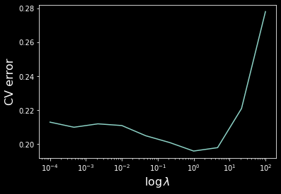
Hence we have $\lambda \approx 1$ achieving the lowest validation error.

testerr = lrerrorrate(phi(test_x), test_y, trainlr(phi(train_x), train_y, bestl))
print(f"lambda = {bestl}, test error = {testerr}")

Producing the test error of $\boxed{5.1\%}$, not bad!

AutoGluon

For comparison, let’s see the performance of an AutoML library which will automatically process the data, train and combine a range of models.

from autogluon.tabular import TabularPredictor, TabularDataset
train_data, test_data = TabularDataset(data[:3000]), TabularDataset(data[3000:])
predictor = TabularPredictor(label=57).fit(train_data)
y_pred = predictor.predict(test_data.iloc[:, :57])
testerr = np.sum(test_y.transpose()*y_pred.to_numpy() < 0)/test_y.shape[0]
print(f"test error = {testerr}")

Yielding test error of $\boxed{3.6\%}$ , beating LR by $1.5\%$ !