Kalman Filter

\(\DeclareMathOperator*{\E}{\mathbb{E}}\) \(\DeclareMathOperator*{\V}{\mathbb{V}}\)

Local level model

One of the simplest state space models is the local level model. Its observation (aka measurement) and state (aka transition) equations are given as

with $t=1,\ldots,n$ and with some initial $x_0\overset{iid}{\sim}\mathcal{N}(a_0, P_0)$. Notice that while the measurements $y_t$ are observed at time $t$, the states $x_t$ are not observed! Given the normality of errors, the model can be rewritten as

and solved “brute force” by maximum likelihood. However, due to serial correlation between $y_t$ this approach can become computationally challenging when $n$ gets large. This is especially true for less trivial state space formulations with more parameters. This is where Kalman Filter comes in!

Kalman Filter

KF permits to estimate the unobserved states $x_t$ given the knowledge of the state equation and the observations $y_t$ as they come in. In fact, KF uses these two sources of information iteratively: at $t-1$, KF uses the state equation to predict the state with $\widehat{x}_ {t\mid t-1}$ and at $t$, once $y_t$ is observed, KF updates the estimate $\widehat{x} _{t\mid t}$ with new measurement information. In parallel, KF also updates and predicts the error associated with the state equation projections – this is necessary to balance off the trust between the two sources of information, state equation prediction vs measurement update.

Some notation

where $k,l \in [1,\ldots, n]$.

The prediction step simply computes the conditional mean and variance of $x_t$

which can readily be computed based on the state equation

The above equations solely leverage the state transition equations to predict where the state might be at time $t$. But then, at time $t$, $y_t$ comes in – how do we update our knowledge about the state once we observe this new measurement?

From a Bayesian perspective, the state prediction estimate forms a prior while the incoming measurement observation lets us define the likelihood. Hence, the update step yields a posterior estimate.

Oops, product of Gaussians.

Fun Fact.
The product of two Gaussian is a scaled Gaussian:
\(\frac{1}{\sqrt{2\pi}\sigma_1} e^{-\left({\frac{x-\mu_1}{\sigma_1}}\right)} \times \frac{1}{\sqrt{2\pi}\sigma_2} e^{-\left({\frac{x-\mu_2}{\sigma_2}}\right)} = c' \times e^{-\left({\frac{x-\mu'}{\sigma'}}\right)^2},\) where
\(\mu' = \mu_1 + \left(\frac{\sigma^2_1}{\sigma^2_1 + \sigma^2_2}\right)(\mu_2 -\mu_1), \quad \sigma'^2 = \left(1-\frac{\sigma^2_1}{\sigma^2_1 + \sigma^2_2}\right) \sigma_1^2.\)

Hence we can rewrite the above density as

with the following equations defining the update step

Kalman gain

The term $k _t := \frac{\widehat{v}^2 _{t\mid t-1}}{\widehat{v}^2 _{t\mid t-1} + \sigma _\epsilon^2}$ is known as Kalman gain. Notice how it balances the information coming from state and measurement signals: if the measurement noise $\sigma _\epsilon^2$ is high, Kalman gain $k _t$ is small, and hence the update equations will place more weight on the information coming from the state transition equations.

Putting everything together, the KF equations for the above local linear model are

Notice the dynamics of uncertainty over time: the state estimate uncertainty $\widehat{v}^2$ increases with each prediction but decreases every time the measurement is observed.

No data – no problem

One of the nicest things about state space models & KF is that the missing data problem is handled naturally. If no $y_t$ is brought in at $t$, one can omit the update step. Then the estimate would be solely determined by the “model”, i.e. by its state transition prediction. From a bayesian standpoint, our posterior estimate is set equal to the prior as no likelihood can be formed.

More general case

We have an $N\times 1$ vector $\mathrm{y}_t$ and an $m\times 1$ state vector $\mathrm{x}_t$. A general state space model can be specified as follows

where $Z_t$ is an $N\times m$ design matrix, $T_t$ is an $m\times m$ transition matrix and $R_t$ is an $m\times g$ selection matrix. Further, it is often assumed that the two errors are uncorrelated

State space modeling is fairly general as several approaches can be formulated in this form, including SARIMAX, VARMAX, unobserved components, factor models, linear exponential smoothing models, etc.

AR(2) Model

An AR(2) model

can be cast into state space form in several ways. For example,

where \(\mathrm{x}_t = \begin{pmatrix} \mathrm{y}_t \\ y_{t-1}\end{pmatrix}\) and we let

and so we have three parameters to estimate: $\phi_1, \phi_2, \sigma^2$.

MA(1) Model

An MA(1) model

can be cast as

where \(\mathrm{x}_t = \begin{pmatrix} \mathrm{y}_t \\ \theta \nu_t \end{pmatrix}\).

ARMA(1,1) Model

An ARMA(1,1) model

can be cast as

where \(\mathrm{x}_t = \begin{pmatrix} \mathrm{y}_t \\ \theta \nu_t \end{pmatrix}\).

General Update & Prediction

Letting \(\widehat{\mathrm{x}}_{k\mid l} := \E(\mathrm{x}_k\mid I_{l})\) and \(P_{k\mid l} := \V(\mathrm{x}_k\mid I_{l})\)

Example & Code

Notation change alert!

Consider another specification as given in wikipedia.

The KF solution script is stolen from given in here.

import numpy as np

class KalmanFilter(object):
    def __init__(self, F = None, B = None, H = None, Q = None, R = None, P = None, x0 = None):

        if(F is None or H is None):
            raise ValueError("Set proper system dynamics.")

        self.n = F.shape[1]
        self.m = H.shape[1]

        self.F = F
        self.H = H
        self.B = 0 if B is None else B
        self.Q = np.eye(self.n) if Q is None else Q
        self.R = np.eye(self.n) if R is None else R
        self.P = np.eye(self.n) if P is None else P
        self.x = np.zeros((self.n, 1)) if x0 is None else x0

    def predict(self, u = 0):
        self.x = np.dot(self.F, self.x) + np.dot(self.B, u)
        self.P = np.dot(np.dot(self.F, self.P), self.F.T) + self.Q
        return self.x

    def update(self, z):
        y = z - np.dot(self.H, self.x)
        S = self.R + np.dot(self.H, np.dot(self.P, self.H.T))
        K = np.dot(np.dot(self.P, self.H.T), np.linalg.inv(S))
        self.x = self.x + np.dot(K, y)
        I = np.eye(self.n)
        self.P = np.dot(np.dot(I - np.dot(K, self.H), self.P), 
        	(I - np.dot(K, self.H)).T) + np.dot(np.dot(K, self.R), K.T)

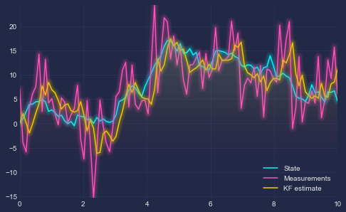
Suppose we make the data generating process look like

for $t=1,\ldots,100$ and try to estimate the simple local level model we started with at the beginning

F = np.array([1]).reshape(1, 1)
H = np.array([1]).reshape(1, 1)
Q = np.array([1]).reshape(1, 1)
R = np.array([5]).reshape(1, 1)

# DGP
time = np.linspace(0, 10, 100)
x = np.zeros(100)
for t in range(99):
    x[t+1] = x[t] + np.random.normal(0, 1)
measurements = x + np.random.normal(0, 5, 100)

kf = KalmanFilter(F = F, H = H, Q = Q, R = R)
predictions = []

for z in measurements:
    predictions.append(np.dot(H,  kf.predict())[0])
    kf.update(z)

import matplotlib.pyplot as plt
plt.plot(time, x, label = 'State')
plt.plot(time, measurements, label = 'Measurements')
plt.plot(time, np.array(predictions), label = 'KF estimate')
plt.legend()
plt.show()

We get the following result